Plotting your data • mort

Plotting your data is invaluable in exploring and understanding your data. The mortsplot() function plots your data using ggplot2, as well as some automatically calculated presets that should generate useful and functional plots for most datasets. All the plots in the vignettes were generated using mortsplot(). ggplot2 is suggested by mort, but is not required for installation. To use mortsplot(), it is the responsibility of the user to install and load ggplot2.

Basic plotting of residence events

A basic plot can be quickly generated using a dataframe with residence events, and the same arguments that are used in other morts functions:

plot<-mortsplot(data=events,type="mort",ID="ID",station="Station.Name")
plot

Customizing

Because mortsplot() calls ggplot(), the plot can be customized by adding additional arguments as you would with any other ggplot2 object. For example, you can remove the legend by calling:

plot<-plot+
  theme(legend.position="none")
plot

Interactive plots

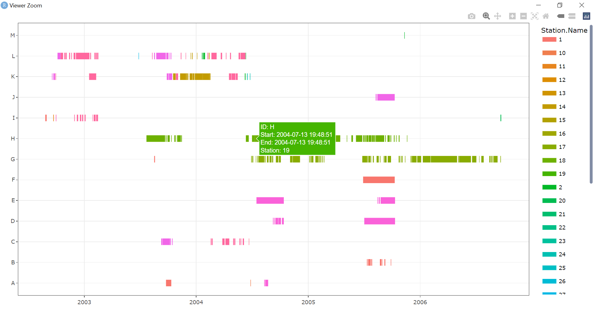
Interactive plots can be generated easily with the interactive argument in mortsplot():

plot<-mortsplot(data=events,type="mort",ID="ID",station="Station.Name",interactive=TRUE)
plot

Zooming and scrolling around the interactive plot are possible (using the toolbar at the top right corner), as well as changing the visibility of stations (by clicking on the station names). Information about each residence event appears when the cursor is moved over the beginning or end of a residence event.

When interactive=TRUE, mortsplot() calls ggplotly() from plotly. The same result can be achieved by building a non-interactive plot with mortsplot() and calling ggplotly() directly:

interactive_plot<-ggplotly(plot)
interactive_plot

Options

There are several options to customize mortsplot() plots:

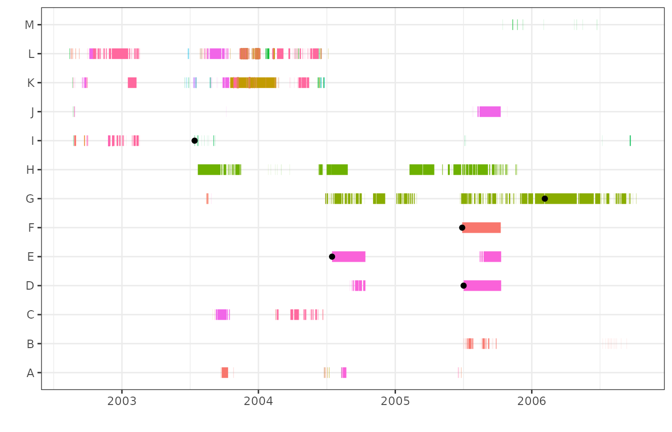
Add flagged mortalities

After potential mortalities have been identified, they can be added to the plot as black points with the morts argument:

plot<-mortsplot(data=events,type="mort",ID="ID",station="Station.Name",morts=morts)

Seasonality

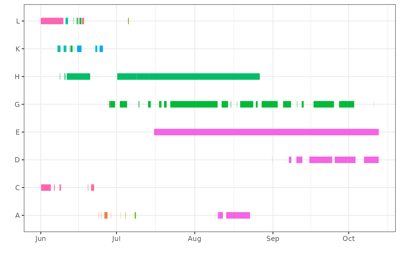
To plot specific seasons or periods of interest, seasonality can be applied using the arguments season.start and season.end. These arguments are used in the same way as for season() (see the Seasonality vignette) or when seasonality is applied in morts() (see the Identifying potential mortalities vignette).

To apply seasonality, the arguments residences and units must also be provided, in the same manner as they are in other morts functions.

plot<-mortsplot(data=events,type="mort",ID="ID",station="Station.Name",
                residences="auto",units="auto",
                season.start="2004-06-01",season.end="2004-10-31")

Facetting

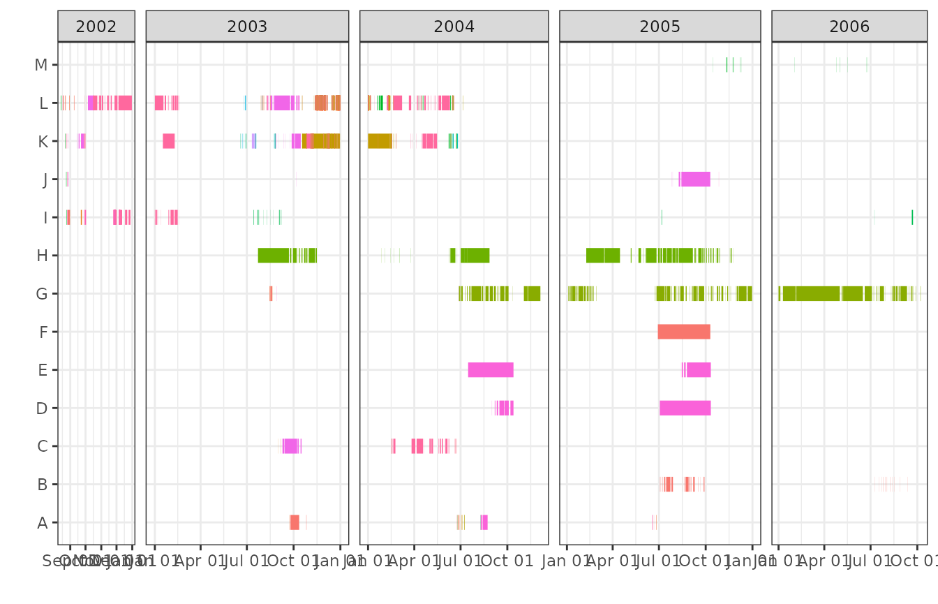
Depending on the duration of your dataset, the number of animals, and if seasonality is applied, it may be desirable to facet the plot by year or season. This is done by including the argument facet=TRUE, along with the arguments for seasonality (see above). The plot will automatically facet along the x axis, with each specified season forming a panel.

plot<-mortsplot(data=events,type="mort",ID="ID",station="Station.Name",facet=TRUE,
                season.start=c("2004-06-01","2004-10-01"),
                season.end=c("2004-06-30","2004-10-31"))

For multi-year datasets, it is also possible to facet by year instead of user-defined seasons.

plot<-mortsplot(data=events,type="mort",ID="ID",station="Station.Name",
                facet=TRUE,facet.by="year")

The default is to position panels along the x axis. The facet axis can be changed using the facet.axis argument. Note that the y-axis can only be used if facetting by year.

plot<-mortsplot(data=events,type="mort",ID="ID",station="Station.Name",
                facet=TRUE,facet.by="year",facet.axis="y")

Exclude single detections

In mortsplot(), the argument singles specifies if single detections are plotted. The default setting is singles=TRUE, to include single detections. If single detections are included, they would normally not be visible in the plot because their duration is 0. mortsplot() performs a simple calculation to determine a dummy duration to assign to single detections. The dummy duration depends on the scale of the plot, and is long enough to be visible but short enough that it should not interfere with the visibility of other residence events.

Source code

You may have tried the mortsplot() function, adding additional arguments as above, and the options above, and you find that mortsplot() still does not provide practical plots for your dataset. If this is the case and you want to use some aspects of the plot, please access the source code at github.com/rosieluain/mort or entering the following into the console:

View(mortsplot)