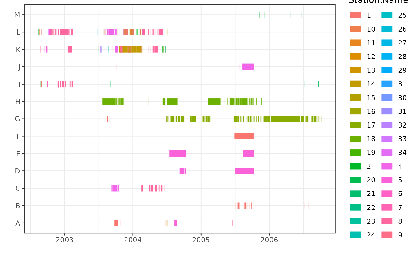
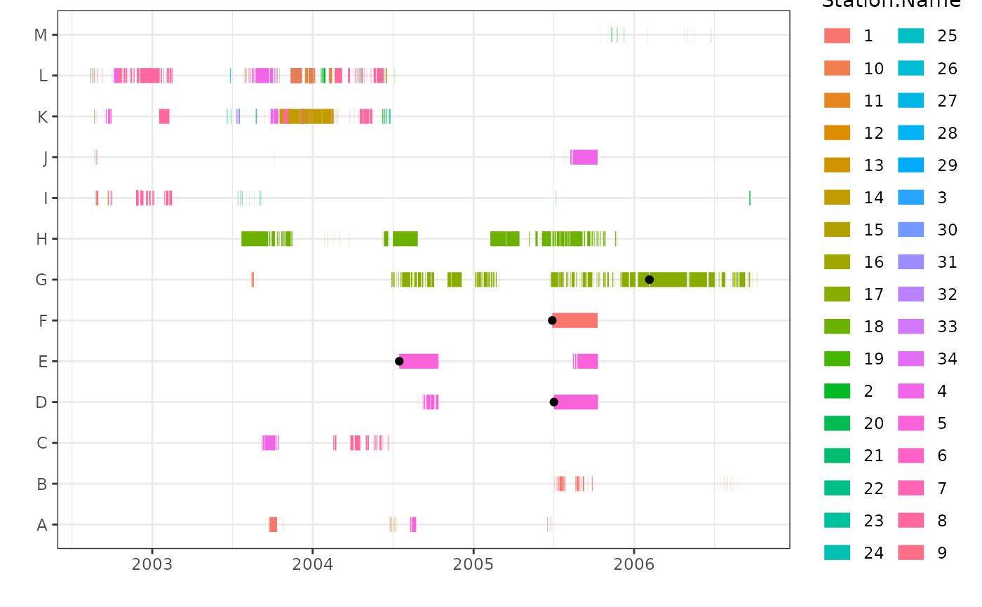
Plot residence events, with the option of plotting identified mortalities. Plotting uses ggplot2. Interactive option also uses plotly.
mortsplot(
  data,
  type,
  ID,
  station,
  res.start = "auto",
  res.end = "auto",
  morts = NULL,
  singles = TRUE,
  interactive = FALSE,
  residences = NULL,
  units = NULL,
  season.start = NULL,
  season.end = NULL,
  facet = FALSE,
  facet.axis = "x",
  facet.by = "season",
  verbose = TRUE
)
Arguments
- data
a dataframe of residence events. Residence events must include tag ID, location name, start time, and end time.
- type
the method used to generate the residence events. Options are "mort", "actel", "glatos", "vtrack", or "manual".
- ID
a string of the name of the column in
datathat holds the tag or sample IDs.- station
a string of the name of the column in
datathat holds the station name or receiver location.- res.start
a string of the name of the column in
datathat holds the start date and time. Must be specified and in POSIXt or character in the format YYYY-mm-dd HH:MM:SS iftype="manual".- res.end
a string of the name of the column in
datathat holds the end date and time. Must be specified and in POSIXt or character in the format YYYY-mm-dd HH:MM:SS iftype="manual".- morts
a dataframe containing potential mortalities. The dataframe must have the same ID, station, res.start, res.end, and residences column names as
data.- singles
option to adjust the end times of residence events so single detection events are visible. Adjustment is for visualization purposes only and should not obscure or impact the visualization of other residence events.
- interactive
option to generate an interactive plot.
- residences
an optional character string with the name of the column in
datathat holds the duration of the residence events. Required if generating an interactive plot or applying season.- units
units of the duration of the residence events in
data. Required if applying season.- season.start
the start date/time(s) of the period of interest. If the period of interest is the same in all study years, must be a character string in format "dd-mm". Otherwise, must be in POSIXt, or a character string in format YYYY-mm-dd HH:MM:SS.
- season.end
the end date/time(s) of the period of interest. If the period of interest is the same in all study years, must be a character string in format "dd-mm". Otherwise, must be in POSIXt, or a character string in format YYYY-mm-dd HH:MM:SS.
- facet
option to facet by year or season. If
TRUE, thenseason.startandseason.endmust be provided.- facet.axis
option to position facets along x or y axis. Options are "x" and "y". Default is "x". Note that
facet.axiscan only be "y" iffacet.by="year".- facet.by
option to facet by "season" (as defined with
season.startandseason.end) or "year". Default is "season".- verbose
option to display updates and progress bar as function is run. Default is TRUE.
Value
a ggplot2 plot. Additional arguments (e.g., formatting axes,
legend, aes, manual colour scales) can be added as for any ggplot2 plot.
If interactive=TRUE,
returns a plotly plot.
Examples
plot<-mortsplot(data=events,type="mort",ID="ID",station="Station.Name")
plot


# With mortalities plotted over residences:
morts<-morts(data=events,type="mort",ID="ID",station="Station.Name",
method="any",verbose=FALSE)
#>
  |
  |                                                                      |   0%
  |
  |======                                                                |   8%
  |
  |============                                                          |  17%
  |
  |==================                                                    |  25%
  |
  |=======================                                               |  33%
  |
  |=============================                                         |  42%
  |
  |===================================                                   |  50%
  |
  |=========================================                             |  58%
  |
  |===============================================                       |  67%
  |
  |====================================================                  |  75%
  |
  |==========================================================            |  83%
  |
  |================================================================      |  92%
  |
  |======================================================================| 100%
  |
  |                                                                      |   0%
  |
  |======                                                                |   8%
  |
  |============                                                          |  17%
  |
  |==================                                                    |  25%
  |
  |=======================                                               |  33%
  |
  |=============================                                         |  42%
  |
  |===================================                                   |  50%
  |
  |=========================================                             |  58%
  |
  |===============================================                       |  67%
  |
  |====================================================                  |  75%
  |
  |==========================================================            |  83%
  |
  |================================================================      |  92%
  |
  |======================================================================| 100%

plot<-mortsplot(data=events,type="mort",ID="ID",station="Station.Name",
morts=morts)
plot
