Seasonality

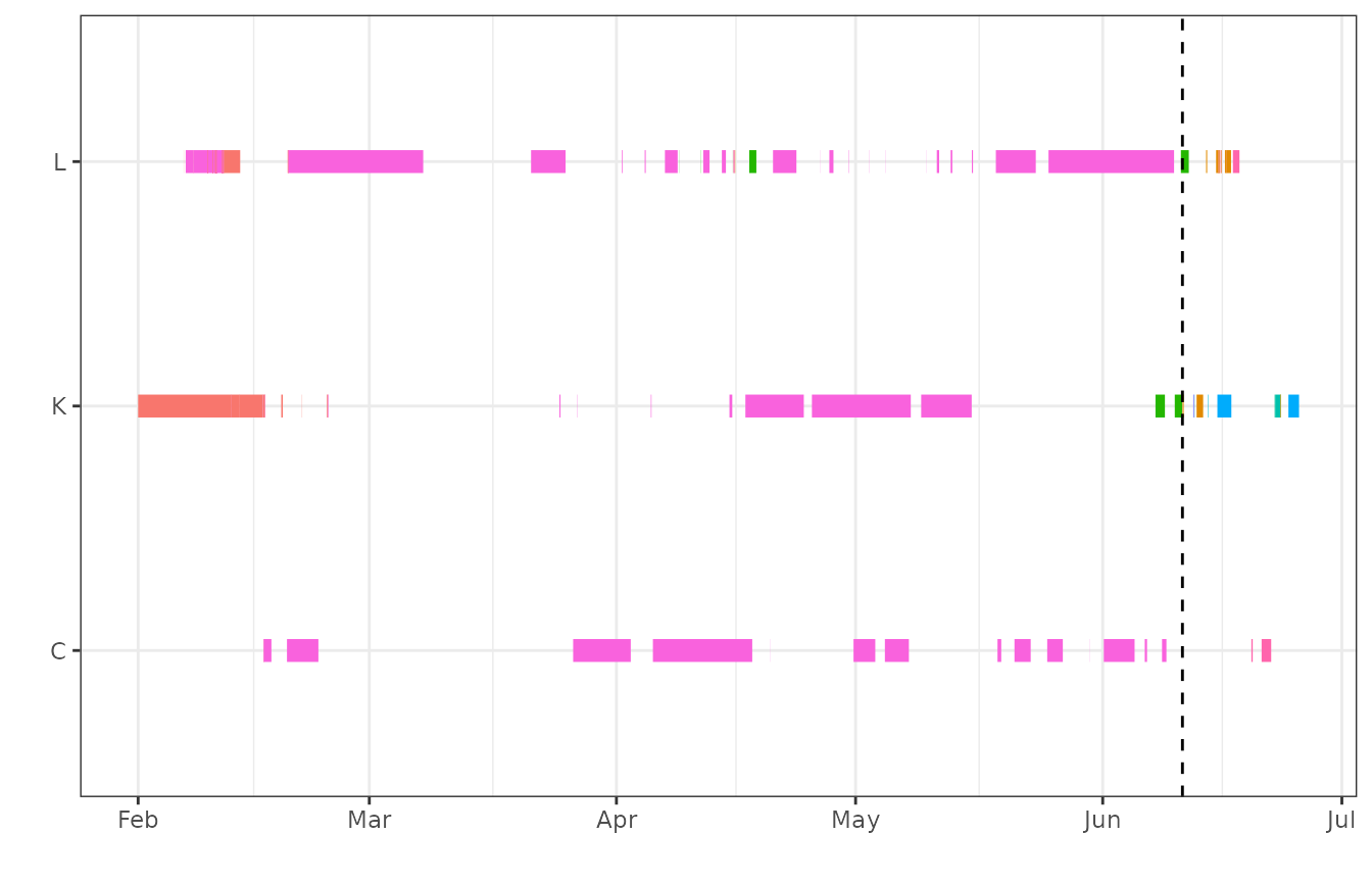
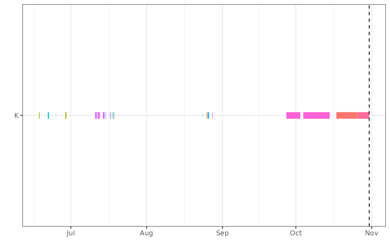
Some species may exhibit seasonal patterns in movement. For example, in the plot below, there is reduced movement during the ice-covered season (before the dashed line), with associated long residence events. In summer (after the dashed line), when movement activity increases, residence events may also increase in number and frequency.

If this is the case, the long residence events will likely increase thresholds for morts(). Animals that do not move during the summer months, and are likely mortalities, may then not exceed the threshold. For this reason, there is the option to define seasons or periods of interest in morts(). If seasonality is applied, then both thresholds and mortalities are identified only using data or residence events from the specified periods.

Applying seasonality

To apply seasonality, the arguments season.start and season.end must be specified. There are two ways that the start and end can be specified. If the study takes place over multiple years and the season or period of interest is the same in all years, start and end can be specified as a day and month using a character string in format dd-mm.

day_month<-morts(data=events,type="mort",ID="ID",station="Station.Name",
                 season.start="01-06", season.end="31-10")

Alternatively, if there are multiple periods of interest within a year, and/or the periods change from year to year, start and end can be specified. Start and end can be specified either as POSIXt date and times, or as character strings in the format YYYY-mm-dd HH:MM:SS.

full_date<-morts(data=events,type="mort",ID="ID",station="Station.Name",
                 season.start=c("2003-06-01","2004-06-05"),
                 season.end=c("2003-10-31","2004-10-15"))

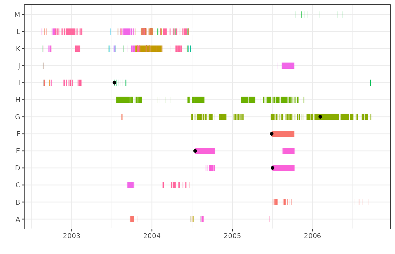
Here is how mortalities would be identified, using method="all" and no seasonality. The black points indicate the time of a potential mortality.

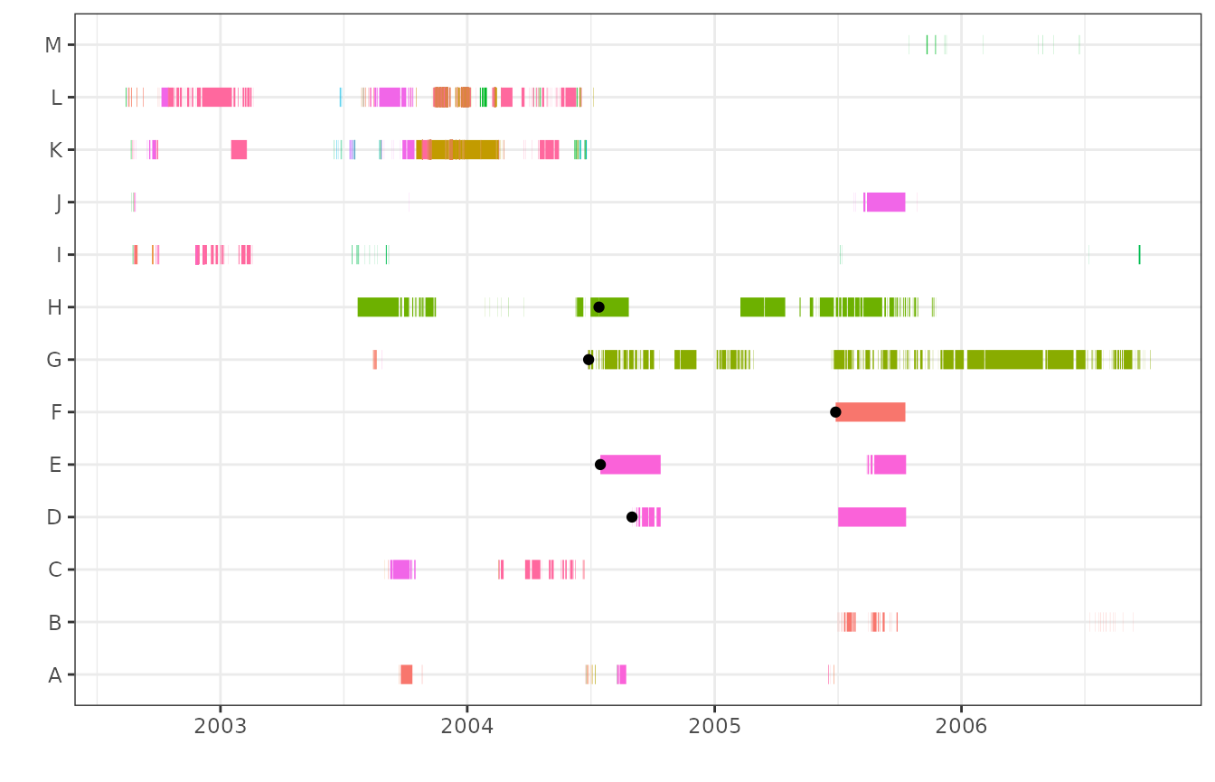
And here is when seasonality is included:

Note that animal I is not flagged as a potential mortality when seasonality is applied. However, animal I would likely be flagged if the infrequent() function was used in addition to morts().

overlap argument

There is an optional argument when applying seasonality. The overlap argument specifies whether residence events that overlap (i.e., start before and end after) the season start or end are included in full, or if the overlapping residence events are truncated at the specified start and/or end. The default is overlap=TRUE, which keeps the full residence events, as in the examples above. To truncate the residence events, use overlap=FALSE.

no_overlap<-morts(data=events,type="mort",ID="ID",station="Station.Name",
                 season.start="2003-06-01", season.end="2003-10-31",
                 season.overlap=FALSE)

Here is an example of residence events with overlap (overlap=TRUE):

Here is an example of residence events without overlap (overlap=FALSE):

season() function

If you are interested in exploring residence events after applying seasonality, the season() function, which is called by morts(), is also available as a standalone function. The arguments for season() are the same as those for the other functions.

season.data<-season(data=events,type="mort",ID="ID",station="Station.Name",
                    season.start="2003-06-01", season.end="2003-10-31")